3. In-Depth Guide: Model Training & Evaluation
This guide covers the model training process in detail, including dataset registration, configuration for single and multi-class problems, and how to evaluate model performance.
3.1. The Training Workflow
1. Registering Datasets
Before training can commence, you must register your tiled training and validation datasets with Detectron2.
For single-class datasets:
from detectree2.models.train import register_train_data

train_location = "/path/to/Danum/tiles/train/"
register_train_data(train_location, 'Danum', val_fold=5)
For multi-class datasets, you must also provide the path to the class_to_idx.json file you created during data preparation. This ensures the model knows about all possible classes.
from detectree2.models.train import register_train_data

train_dir = "/path/to/Danum_lianas/tiles/train"
class_mapping_file = "/path/to/Danum_lianas/tiles/class_to_idx.json"
data_name = "DanumLiana"

register_train_data(train_dir, data_name, val_fold=5, class_mapping_file=class_mapping_file)
The data will be registered as <name>_train and <name>_val (e.g., Danum_train and Danum_val).
2. Configuring the Model
We must supply a base_model from Detectron2’s model_zoo. This loads a backbone that has been pre-trained, which saves time and improves performance.
For single-class training:
from detectree2.models.train import setup_cfg

# Set the base (pre-trained) model from the detectron2 model_zoo
base_model = "COCO-InstanceSegmentation/mask_rcnn_R_101_FPN_3x.yaml"

trains = ("Danum_train", "Paracou_train") # Registered train data
tests = ("Danum_val", "Paracou_val")     # Registered validation data

out_dir = "./train_outputs"

cfg = setup_cfg(base_model, trains, tests, workers=4, eval_period=100, max_iter=3000, out_dir=out_dir)
Alternatively, it is possible to train from one of detectree2’s pre-trained models. This is recommended if you have limited training data.
# Download a pre-trained model
# !wget https://zenodo.org/records/15863800/files/250312_flexi.pth

trained_model = "./250312_flexi.pth"
cfg = setup_cfg(base_model, trains, tests, trained_model, workers=4, eval_period=100, max_iter=3000, out_dir=out_dir)
For multi-class training, you must pass the class_mapping_file to the configuration setup. This automatically registers the correct number of classes with the model.
cfg = setup_cfg(
    base_model="COCO-InstanceSegmentation/mask_rcnn_R_101_FPN_3x.yaml",
    trains=("DanumLiana_train",),
    tests=("DanumLiana_val",),
    max_iter=50000,
    eval_period=50,
    base_lr=0.003,
    out_dir="./liana_outputs",
    class_mapping_file=class_mapping_file
)
3. Running the Trainer
Once configured, you can start the training. The trainer includes “early stopping” via the patience parameter, which stops training if validation accuracy does not improve for a set number of epochs.
from detectree2.models.train import MyTrainer

trainer = MyTrainer(cfg, patience=5)
trainer.resume_or_load(resume=False)
trainer.train()
3.2. Data Augmentation
Data augmentation artificially increases the size of the training dataset by applying random transformations to the input data, which helps improve model generalization.
By default, random rotations and flips will be performed on input images.
augmentations = [
   T.RandomRotation(angle=[0, 360], expand=False),
   T.RandomFlip(prob=0.5, horizontal=True, vertical=False),
]
If the input data is RGB, additional augmentations will be applied to adjust the brightness, contrast, saturation, and lighting of the images.
# Additional augmentations for RGB images
if cfg.IMGMODE == "rgb":
   augmentations.extend([
         T.RandomBrightness(0.7, 1.5),
         T.RandomLighting(0.7),
         T.RandomContrast(0.6, 1.3),
         T.RandomSaturation(0.8, 1.4)
   ])
There are three resizing modes for the input data: fixed, random, and rand_fixed, set in the setup_cfg function.
fixed: Resizes images to a fixed width/height (e.g., 1000 pixels). Efficient but less flexible.
random: Randomly resizes images between 0.6x and 1.4x their original size. Helps the model learn to detect objects at different scales.
rand_fixed: Randomly resizes images but constrains them to a fixed pixel range (e.g., 600-1400 pixels). A good compromise between flexibility and memory usage.
3.3. Post-Training Analysis
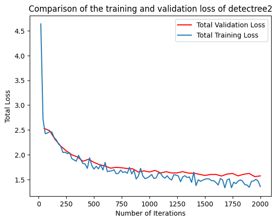
It is important to check that the model has converged and is not overfitting. You can do this by plotting the training and validation loss from the metrics.json file output by the trainer.
import json
import matplotlib.pyplot as plt
from detectree2.models.train import load_json_arr

experiment_folder = "./train_outputs"
experiment_metrics = load_json_arr(experiment_folder + '/metrics.json')

plt.plot(
   [x['iteration'] for x in experiment_metrics if 'validation_loss' in x],
   [x['validation_loss'] for x in experiment_metrics if 'validation_loss' in x], label='Total Validation Loss', color='red')
plt.plot(
   [x['iteration'] for x in experiment_metrics if 'total_loss' in x],
   [x['total_loss'] for x in experiment_metrics if 'total_loss' in x], label='Total Training Loss')

plt.legend(loc='upper right')
plt.title('Comparison of the training and validation loss of detectree2')
plt.ylabel('Total Loss')
plt.xlabel('Number of Iterations')
plt.show()
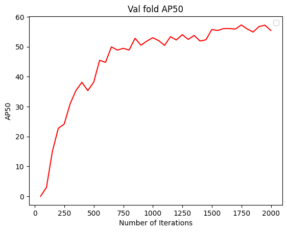
To understand how segmentation performance improves, you can also plot the AP50 score over iterations.
plt.plot(
   [x['iteration'] for x in experiment_metrics if 'bbox/AP50' in x],
   [x['bbox/AP50'] for x in experiment_metrics if 'bbox/AP50' in x], label='Validation AP50')

plt.legend(loc='lower right')
plt.title('Validation AP50 over training iterations')
plt.ylabel('AP50')
plt.xlabel('Number of Iterations')
plt.show()
3.4. Evaluating Model Performance
Coming soon! See Colab notebook for an example routine (detectree2/notebooks/colab/evaluationJB.ipynb).
Performance Metrics Explained
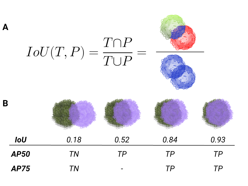
In instance segmentation, AP50 refers to the Average Precision at an Intersection over Union (IoU) threshold of 50%.
IoU (Intersection over Union): IoU measures the overlap between the predicted segmentation mask and the ground truth mask. It is calculated as the area of overlap divided by the area of union.
AP50: A predicted object is considered a true positive if its IoU with a ground truth mask is >= 0.5 (50%). AP50 is the average precision calculated at this 50% threshold. It is a standard metric for evaluating how well a model detects objects.