1. Getting Started: Your First Prediction
This tutorial goes through the essential steps of single-class (tree) detection and delineation from RGB data. The goal is to provide a concise, end-to-end walkthrough to get you from an orthomosaic to a final crown prediction map.
Example data that can be used in this tutorial is available here.
The key steps are:
Preparing data
Training a model
Making landscape-level predictions
Before getting started ensure detectree2 is installed:
(.venv) $ pip install torch torchvision
(.venv) $ pip install 'git+https://github.com/facebookresearch/detectron2.git'
(.venv) $ pip install detectree2
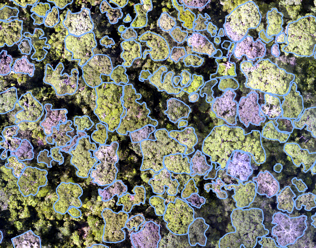
To train a model you will need an orthomosaic (as <orthomosaic>.tif) and
corresponding tree crown polygons that are readable by Geopandas
(e.g. <crowns_polygon>.gpkg, <crowns_polygon>.shp). For the best
results, manual crowns should be supplied as dense clusters rather than
sparsely scattered across in the landscape. The method is designed to make
predictions across the entirety of the supplied tiles and assumes training
tiles are comprehensively labelled. If the network is shown scenes that are
incompletely labelled, it may replicate that in its predictions. See
below for an example of the required input crowns and image.
If you would just like to make predictions on an orthomosaic with a pre-trained
model from the model_garden, skip to Making Landscape-Level Predictions.
1.1. Preparing Data
First, we tile our large orthomosaic and crown data into smaller images suitable for training.
We call functions from detectree2’s tiling module.
from detectree2.preprocessing.tiling import tile_data, to_traintest_folders
import geopandas as gpd
import rasterio
Set up the paths to the orthomosaic and corresponding manual crown data.
# Set up input paths
site_path = "./Paracou" # Example path
img_path = site_path + "/rgb/Paracou_RGB_2016_10cm.tif"
crown_path = site_path + "/crowns/UpdatedCrowns8.gpkg"

# Read in crowns and match CRS to the image
data = rasterio.open(img_path)
crowns = gpd.read_file(crown_path)
crowns = crowns.to_crs(data.crs.data)
Set up the tiling parameters and tile the data. The tile_data function, when crowns is supplied, will only retain tiles that contain a certain coverage of training data.
# Set tiling parameters
buffer = 30
tile_width = 40
tile_height = 40
threshold = 0.6
out_dir = site_path + "/tiles/"

# Tile the data for training
tile_data(img_path, out_dir, buffer, tile_width, tile_height, crowns, threshold, mode="rgb")
Finally, partition the tiled data into train and test sets.
# Create train/test folders
to_traintest_folders(out_dir, out_dir, test_frac=0.15)
1.2. Training a Model
Before training can commence, it is necessary to register the training data.
from detectree2.models.train import register_train_data, MyTrainer, setup_cfg

train_location = out_dir + "/train/"
register_train_data(train_location, 'Paracou', val_fold=5)
Next, we configure the model. We use a base_model from Detectron2’s model zoo, which provides a pre-trained backbone to speed up training.
# Set the base (pre-trained) model from the detectron2 model_zoo
base_model = "COCO-InstanceSegmentation/mask_rcnn_R_101_FPN_3x.yaml"

trains = ("Paracou_train",) # Registered train data
tests = ("Paracou_val",)   # Registered validation data

model_output_dir = "./train_outputs"

cfg = setup_cfg(base_model, trains, tests, workers=4, eval_period=100, max_iter=3000, out_dir=model_output_dir)
Now, we can start training.
trainer = MyTrainer(cfg, patience = 5)
trainer.resume_or_load(resume=False)
trainer.train()
Training outputs, including model weights, will be stored in model_output_dir.
1.3. Making Landscape-Level Predictions
To make predictions on a full orthomosaic, we first tile it into manageable pieces.
from detectree2.models.predict import predict_on_data
from detectree2.models.outputs import project_to_geojson, stitch_crowns, clean_crowns
from detectron2.engine import DefaultPredictor

# Path to the full orthomosaic
img_path = site_path + "/rgb/Paracou_RGB_2016_10cm.tif"
pred_tiles_path = site_path + "/tiles_pred/"

# Specify tiling parameters (should be similar to training)
buffer = 30
tile_width = 40
tile_height = 40
tile_data(img_path, pred_tiles_path, buffer, tile_width, tile_height)
Point to your trained model, set up the configuration, and make predictions on the tiles.
# You can use your own trained model or download a pre-trained one
# !wget https://zenodo.org/records/15863800/files/250312_flexi.pth

trained_model = "./230103_randresize_full.pth"
cfg = setup_cfg(update_model=trained_model)
predictor = DefaultPredictor(cfg)
predict_on_data(pred_tiles_path, predictor)
Once predictions are made on the tiles, project them back into geographic space, stitch them together, and clean up overlapping predictions.
# Project tile predictions to geo-referenced crowns
project_to_geojson(pred_tiles_path, pred_tiles_path + "predictions/", pred_tiles_path + "predictions_geo/")

# Stitch and clean crowns
crowns = stitch_crowns(pred_tiles_path + "predictions_geo/")
clean = clean_crowns(crowns, 0.6, confidence=0.5) # Filter low-confidence and overlapping crowns
1.4. Saving and Visualizing Your Crowns
Finally, save your cleaned-up crown map to a file.
# Simplify geometries for easier editing in GIS software
clean = clean.set_geometry(clean.simplify(0.3))

# Save to file
clean.to_file(site_path + "/crowns_out.gpkg", driver="GPKG")
You can now view the crowns_out.gpkg file in QGIS or ArcGIS to see your results.