2. In-Depth Guide: Data Preparation

This guide provides a detailed look at preparing your data for use with detectree2, covering everything from basic tiling to advanced options and multi-class data handling.

2.1. Core Tiling Concepts (RGB & Multispectral)

An example of the recommended file structure when training a new model is as follows:

├── Danum                                       (site directory)
│   ├── rgb
│   │   └── Dan_2014_RGB_project_to_CHM.tif     (RGB orthomosaic in local UTM CRS)
│   └── crowns
│       └── Danum.gpkg                          (Crown polygons readable by geopandas e.g. Geopackage, shapefile)
│
└── Paracou                                     (site directory)
    ├── rgb
    │   ├── Paracou_RGB_2016_10cm.tif           (RGB orthomosaic in local UTM CRS)
    │   └── Paracou_RGB_2019.tif                (RGB orthomosaic in local UTM CRS)
    ├── ms
    │   └── Paracou_MS_2016.tif                 (Multispectral orthomosaic in local UTM CRS)
    └── crowns
        └── UpdatedCrowns8.gpkg                 (Crown polygons readable by geopandas e.g. Geopackage, shapefile)

Here we have two sites available to train on (Danum and Paracou). Several site directories can be included in the training and testing phase (but only a single site directory is required). If available, several RGB orthomosaics can be included in a single site directory (see e.g Paracou -> RGB).

For Paracou, we also have a multispectral scan available (5-bands). For this data, the mode parameter in the tile_data function should be set to "ms". This calls a different routine for tiling the data that retains the .tif format instead of converting to .png as in the case of rgb. This comes at a slight expense of speed later on but is necessary to retain all the multispectral information.

from detectree2.preprocessing.tiling import tile_data
import geopandas as gpd
import rasterio

# Set up input paths
site_path = "/path/to/data/Paracou"
img_path = site_path + "/rgb/2016/Paracou_RGB_2016_10cm.tif"
crown_path = site_path + "/crowns/220619_AllSpLabelled.gpkg"

data = rasterio.open(img_path)
crowns = gpd.read_file(crown_path)
crowns = crowns.to_crs(data.crs.data)

# Set tiling parameters
buffer = 30
tile_width = 40
tile_height = 40
threshold = 0.6
out_dir = site_path + "/tiles/"

tile_data(img_path, out_dir, buffer, tile_width, tile_height, crowns, threshold, mode="rgb")

Warning

If tiles are outputting as blank images set dtype_bool = True in the tile_data function. This is a bug and we are working on fixing it.

Note

You will want to relax the threshold value if your trees are sparsely distributed across your landscape or if you want to include non-forest areas (e.g. river, roads). Remember, detectree2 was initially designed for dense, closed canopy forests so some of the default assumptions will reflect that and parameters will need to be adjusted for different systems.

2.2. Advanced Tiling Options

The tile_data function exposes many parameters to control how tiles are created. Here are some of the most useful ones in more detail:

• tile_placement: Choose how tile origins are generated.

  • "grid" (default): Lays tiles on a fixed grid across the image bounds. Fast and predictable.

  • "adaptive": A more efficient method for training. It works by first creating a single polygon that is the union of all your training crowns, then intelligently places tiles only in rows that intersect this polygon. This avoids creating empty tiles in areas where you have no training data. Requires supplying crowns; if crowns is None, it falls back to "grid" with a warning.

• overlapping_tiles: When True, adds a second set of tiles shifted by half a tile’s width and height, creating a “checkerboard” pattern. This is useful for ensuring crowns that fall on a tile boundary are fully captured in at least one tile and can help reduce prediction artifacts at tile edges.

• ignore_bands_indices: Zero-based indices of bands to skip (multispectral only). These bands are ignored both when computing image statistics and when writing the output tiles. For example, to exclude band 0 and band 4 in a 5-band raster, pass ignore_bands_indices=[0, 4].

• nan_threshold: The maximum proportion of a tile that can be NaN (or other no-data values) before it is discarded.

• use_convex_mask: When True, this creates a tight “wrapper” polygon (a convex hull) around all the training crowns within a tile. Any pixels outside this wrapper are masked out. This is a way to reduce noise by forcing the model to ignore parts of the tile that are far from any labeled object.

• enhance_rgb_contrast: When True (for RGB images only), this applies a percentile contrast stretch. It calculates the 0.2 and 99.8 percentile pixel values and rescales the image to a 1-255 range. This is effective for normalizing hazy, dark, or washed-out imagery. It allows the model to more easily differentiate between tree crowns. 0 is reserved for masked-out areas.

• additional_nodata: Provide a list of pixel values that should be treated as “no data”. This is a data cleaning tool for real-world rasters that may have multiple invalid or uncommon values (e.g., -9999, 0, 65535) from sensor errors or previous processing steps.

• mask_path: Path to a vector file (e.g., a GeoPackage) that defines your area of interest. If provided, no tiles will be created outside of this area.

• multithreaded: When True, uses multiple CPU cores to process tiles in parallel, significantly speeding up the tiling process for large orthomosaics. Currently, this can cost a linear amount of added memory.

2.3. Practical Recipes for Tiling

Recipe 1: Batch Tiling from Multiple Orthomosaics

To create a larger, more diverse training dataset, you can tile data from several orthomosaics at once and combine them into a single output directory. This can be done by iterating through your data sources in Python.

from detectree2.preprocessing.tiling import tile_data
import geopandas as gpd
import rasterio

sites = [
    {
        "img_path": "/path/to/data/SiteA/ortho.tif",
        "crown_path": "/path/to/data/SiteA/crowns.gpkg",
    },
    {
        "img_path": "/path/to-data/SiteB/ortho.tif",
        "crown_path": "/path/to/data/SiteB/crowns.gpkg",
    },
]

output_dir = "/path/to/my-combined-training-data/"

for site in sites:
    # Read crowns and ensure CRS matches the raster
    with rasterio.open(site["img_path"]) as raster:
        crowns = gpd.read_file(site["crown_path"])
        crowns = crowns.to_crs(raster.crs)
        tile_data(
            img_path=site["img_path"],
            out_dir=output_dir,
            crowns=crowns,
            tile_placement="adaptive",
            mode="ms",
            # other parameters...
            buffer=30,
            tile_width=40,
            tile_height=40,
            threshold=0.6,
        )

Recipe 2: Tiling Noisy Multispectral Rasters

This recipe is ideal for large, real-world multispectral datasets that may contain various “no data” artifacts.

from detectree2.preprocessing.tiling import tile_data
import geopandas as gpd
import rasterio

img_path = "/path/to/your/large_ms_ortho.tif"
crown_path = "/path/to/your/crowns.gpkg"
output_dir = "/path/to/ms_tiles"

# Read crowns and ensure CRS matches the raster
with rasterio.open(img_path) as raster:
    crowns = gpd.read_file(crown_path)
    crowns = crowns.to_crs(raster.crs)

    tile_data(
        img_path=img_path,
        out_dir=output_dir,
        crowns=crowns,
        mode="ms",
        tile_placement="adaptive",
        additional_nodata=[-10000, -20000],
        tile_width=80,
        buffer=10,
        # other parameters...
        tile_height=80,
        threshold=0.6,
    )

2.4. Handling Multi-Class Data

For multi-class problems (e.g., species or disease mapping), you need to provide a class label for each crown polygon.

First, ensure your crowns GeoDataFrame has a column specifying the class for each polygon.

import geopandas as gpd

crown_path = "/path/to/crowns/Danum_lianas_full2017.gpkg"
crowns = gpd.read_file(crown_path)

# The 'status' column here indicates the class of each crown
print(crowns.head())
class_column = 'status'

Next, use the record_classes function to create a class mapping file. This JSON file stores the relationship between class names and their integer indices, which is crucial for training.

from detectree2.preprocessing.tiling import record_classes

out_dir = "/path/to/tiles/"
record_classes(
    crowns=crowns,          # Geopandas dataframe with crowns
    out_dir=out_dir,        # Output directory to save class mapping
    column=class_column,    # Column to be used for classes
    save_format='json'      # Choose between 'json' or 'pickle'
)

This creates a class_to_idx.json in your output directory. When you tile the data, provide the class_column argument to embed this class information into the training tiles.

# Tile the data with class information
tile_data(
    img_path=img_path,
    out_dir=out_dir,
    crowns=crowns,
    class_column=class_column, # Specify the column with class labels
    # ... other parameters
    buffer=30,
    tile_width=40,
    tile_height=40,
    threshold=0.6,
)

2.5. Utilities for Tiled Data

Converting Multispectral Tiles to RGB

If you have multispectral (MS) tiles but want to use them with an RGB-trained model or simply visualize them easily, you can use the create_RGB_from_MS utility. This function converts a folder of MS tiles into a new folder of 3-band RGB tiles.

Note

This utility is very powerful. It not only converts the images but also copies all .geojson annotation files and the train/test folder structure, automatically updating the image paths inside the .geojson files to point to the new RGB .png files.

The function offers two conversion methods: - conversion="pca": Performs a Principal Component Analysis to find the 3 most important components and maps them to R, G, and B. This is great for visualization. - conversion="first-three": Simply takes the first three bands of the MS image.

Here is how you would use it in Python:

from detectree2.preprocessing.tiling import create_RGB_from_MS

# Path to the folder containing your multispectral .tif tiles
ms_tile_folder = "/path/to/ms_tiles/"

# Path for the new RGB tiles
rgb_output_folder = "/path/to/rgb_tiles_from_ms/"

# Convert the tiles using PCA
create_RGB_from_MS(
    tile_folder_path=ms_tile_folder,
    out_dir=rgb_output_folder,
    conversion="pca"
)

Splitting Data into Train/Test/Validation Folds

After tiling, send geojsons to a train folder (with sub-folders for k-fold cross validation) and a test folder.

from detectree2.preprocessing.tiling import to_traintest_folders

data_folder = "/path/to/tiles/"
to_traintest_folders(data_folder, data_folder, test_frac=0.15, strict=False, folds=5)

Note

If strict=True, the to_traintest_folders function will automatically remove training/validation geojsons that have any overlap with test tiles (including the buffers), ensuring strict spatial separation of the test data. However, this can remove a significant proportion of the data available to train on. If validation accuracy is a sufficient test of model performance, you can either not create a test set (test_frac=0) or allow for overlap in the buffers between test and train/val tiles (strict=False).

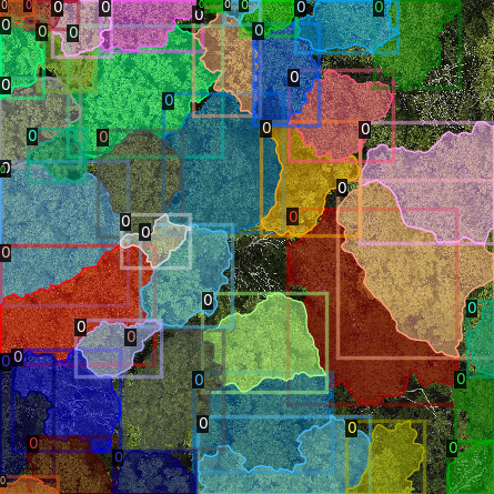
2.6. Visually Inspecting Your Tiles

It is recommended to visually inspect the tiles before training to ensure that the tiling has worked as expected and that crowns and images align. This can be done with the inbuilt detectron2 visualisation tools. For RGB tiles (.png), the following code can be used to visualise the training data.

from detectron2.data import DatasetCatalog, MetadataCatalog
from detectron2.utils.visualizer import Visualizer
from detectree2.models.train import combine_dicts, register_train_data
import random
import cv2
from PIL import Image

name = "Danum"
train_location = "/content/drive/Shareddrives/detectree2/data/" + name + "/tiles_" + appends + "/train"
dataset_dicts = combine_dicts(train_location, 1) # The number gives the fold to visualise
trees_metadata = MetadataCatalog.get(name + "_train")

for d in dataset_dicts:
   img = cv2.imread(d["file_name"])
   visualizer = Visualizer(img[:, :, ::-1], metadata=trees_metadata, scale=0.3)
   out = visualizer.draw_dataset_dict(d)
   image = cv2.cvtColor(out.get_image()[:, :, ::-1], cv2.COLOR_BGR2RGB)
   display(Image.fromarray(image))

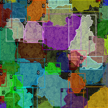
Alternatively, with some adaptation the detectron2 visualisation tools can also be used to visualise the multispectral (.tif) tiles.

import rasterio
from detectron2.utils.visualizer import Visualizer
from detectree2.models.train import combine_dicts
from detectron2.data import DatasetCatalog, MetadataCatalog
from PIL import Image
import numpy as np
import cv2
import matplotlib.pyplot as plt
from IPython.display import display

val_fold = 1
name = "Paracou"
tiles = "/tilesMS_" + appends + "/train"
train_location = "/content/drive/MyDrive/WORK/detectree2/data/" + name + tiles
dataset_dicts = combine_dicts(train_location, val_fold)
trees_metadata = MetadataCatalog.get(name + "_train")

# Function to normalize and convert multi-band image to RGB if needed
def prepare_image_for_visualization(image):
   if image.shape[2] == 3:
      # If the image has 3 bands, assume it's RGB
      image = np.stack([
            cv2.normalize(image[:, :, i], None, 0, 255, cv2.NORM_MINMAX)
            for i in range(3)
      ], axis=-1).astype(np.uint8)
   else:
      # If the image has more than 3 bands, choose the first 3 for visualization
      image = image[:, :, :3]  # Or select specific bands
      image = np.stack([
            cv2.normalize(image[:, :, i], None, 0, 255, cv2.NORM_MINMAX)
            for i in range(3)
      ], axis=-1).astype(np.uint8)

   return image

# Visualize each image in the dataset
for d in dataset_dicts:
   with rasterio.open(d["file_name"]) as src:
      img = src.read()  # Read all bands
      img = np.transpose(img, (1, 2, 0))  # Convert to HWC format
      img = prepare_image_for_visualization(img)  # Normalize and prepare for visualization

   visualizer = Visualizer(img[:, :, ::-1]*10, metadata=trees_metadata, scale=0.5)
   out = visualizer.draw_dataset_dict(d)
   image = out.get_image()[:, :, ::-1]
   display(Image.fromarray(image))