2. Tutorial
This tutorial goes through the steps of single class (tree) detection and delineation from RGB and multispectral data. A guide to multiclass prediction (e.g. species mapping, disease mapping) is coming soon. Example data that can be used in this tutorial is available here.
The key steps are:
Preparing data
Training models
Evaluating model performance
Making landscape level predictions
Before getting started ensure detectree2 is installed through
(.venv) $pip install git+https://github.com/PatBall1/detectree2.git
To train a model you will need an orthomosaic (as <orthomosaic>.tif) and
corresponding tree crown polygons that are readable by Geopandas
(e.g. <crowns_polygon>.gpkg, <crowns_polygon>.shp). For the best
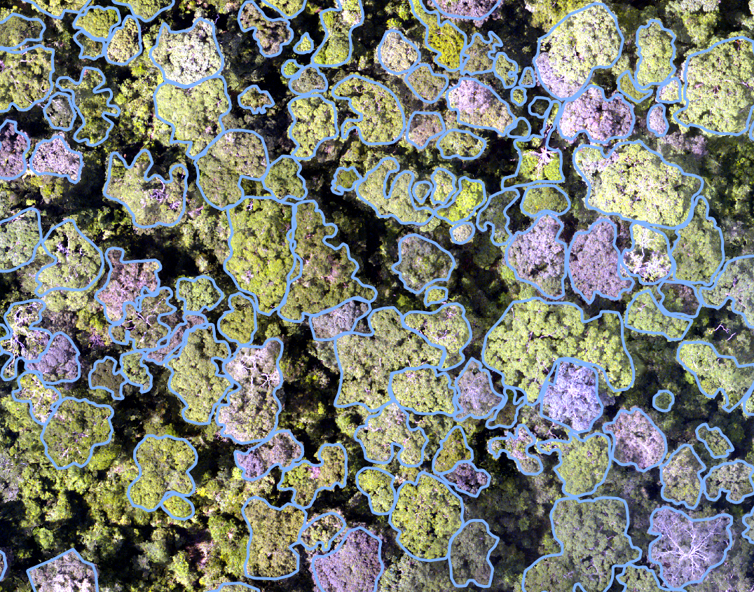
results, manual crowns should be supplied as dense clusters rather than
sparsely scattered across in the landscape. The method is designed to make
predictions across the entirety of the supplied tiles and assumes training
tiles are comprehensively labelled. If the network is shown scenes that are
incompletely labelled, it may replicate that in its predictions. See
below for an example of the required input crowns and image.
If you would just like to make predictions on an orthomosaic with a pre-trained
model from the model_garden, skip to part 2.8 (Generating landscape
predictions).
The data preparation and training process for both RGB and multispectral data is presented here. The process is similar for both data types but there are some key differences that are highlighted. Training a single model on both RGB and multispectral data at the same time is not currently supported. Stick to one data type per model (or stack the RGB bands with the multispectral bands and treat as in the case of multispectral data).
2.1. Preparing data (RGB/multispectral)
An example of the recommended file structure when training a new model is as follows:
├── Danum                                       (site directory)
│   ├── rgb
│   │   └── Dan_2014_RGB_project_to_CHM.tif     (RGB orthomosaic in local UTM CRS)
│   └── crowns
│       └── Danum.gpkg                          (Crown polygons readable by geopandas e.g. Geopackage, shapefile)
│
└── Paracou                                     (site directory)
    ├── rgb
    │   ├── Paracou_RGB_2016_10cm.tif           (RGB orthomosaic in local UTM CRS)
    │   └── Paracou_RGB_2019.tif                (RGB orthomosaic in local UTM CRS)
    ├── ms
    │   └── Paracou_MS_2016.tif                 (Multispectral orthomosaic in local UTM CRS)
    └── crowns
        └── UpdatedCrowns8.gpkg                 (Crown polygons readable by geopandas e.g. Geopackage, shapefile)
Here we have two sites available to train on (Danum and Paracou). Several site directories can be
included in the training and testing phase (but only a single site directory is required).
If available, several RGB orthomosaics can be included in a single site directory (see e.g Paracou -> RGB).
For Paracou, we also have a multispectral scan available (5-bands). For this data, the mode parameter in the
tile_data function should be set to "ms". This calls a different routine for tiling the data that retains the
.tif format instead of converting to .png as in the case of rgb. This comes at a slight expense of speed
later on but is necessary to retain all the multispectral information.
We call functions to from detectree2’s tiling and training modules.
from detectree2.preprocessing.tiling import tile_data, to_traintest_folders
from detectree2.models.train import register_train_data, MyTrainer, setup_cfg
import rasterio
import geopandas as gpd
Set up the paths to the orthomosaic and corresponding manual crown data.
# Set up input paths
site_path = "/content/drive/Shareddrives/detectree2/data/Paracou"
img_path = site_path + "/rgb/2016/Paracou_RGB_2016_10cm.tif"
crown_path = site_path + "/crowns/220619_AllSpLabelled.gpkg"

# Read in the tiff file (this is only necessary to deal with CRS conversion)
# You can skip loading the data if you know crown and mosaic CRS match
data = rasterio.open(img_path)

# Read in crowns (then filter by an attribute if required)
crowns = gpd.read_file(crown_path)
crowns = crowns.to_crs(data.crs.data) # making sure CRS match
Set up the tiling parameters.
The tile size will depend on:
The resolution of your imagery.
Available computational resources.
The detail required on the crown outline.
If using a pre-trained model, the tile size used in training should roughly match the tile size of predictions.
The
modedepends on whether you are tiling 3-band RGB (mode="rgb") data of multispectral data of 4 or more
bands (mode="ms").
# Set tiling parameters
buffer = 30
tile_width = 40
tile_height = 40
threshold = 0.6
appends = str(tile_width) + "_" + str(buffer) + "_" + str(threshold) # this helps keep file structure organised
out_dir = site_path + "/tiles_" + appends + "/"
The total tile size here is 100 m x 100 m (a 40 m x 40 m core area with a surrounding 30 m buffer that overlaps with surrounding tiles). Including a buffer is recommended as it allows for tiles that include more training crowns.
Next we tile the data. The tile_data function, when crowns is supplied, will only retain tiles that contain more
than the given threshold coverage of training data (here 60%). This helps to reduce the chance that the network is
trained with tiles that contain a large number of unlabelled crowns (which would reduce its sensitivity). This value
should be adjusted depending on the density of crowns in the landscape (e.g. 10% may be more appropriate for savannah
type systems or urban environments).
tile_data(img_path, out_dir, buffer, tile_width, tile_height, crowns, threshold, mode="rgb")
Warning
If tiles are outputting as blank images set dtype_bool = True in the tile_data function. This is a bug
and we are working on fixing it. Supplying crown polygons will cause the function to tile for
training (as opposed to landscape prediction which is described below).
Note
You will want to relax the threshold value if your trees are sparsely distributed across your landscape or if you
want to include non-forest areas (e.g. river, roads). Remember, detectree2 was initially designed for dense,
closed canopy forests so some of the default assumptions will reflect that and parameters will need to be adjusted
for different systems.
2.2. Advanced tiling options
The tile_data function exposes a few knobs to better control how tiles are created, especially helpful for large
rasters and multispectral data:
tile_placement: choose how tile origins are generated. -"grid"(default): lays tiles on a fixed grid across the image bounds. Fast and predictable. -"adaptive": concentrates tiles where crowns exist by scanning rows that intersect the union of crowns. Requiressupplying
crowns; ifcrownsisNone, it falls back to"grid"with a warning.overlapping_tiles: whenTrue, adds a second set of tiles shifted by half a tile in X and Y (checkerboard offset). Useful to reduce edge artifacts in predictions, or to capture crowns straddling tile boundaries. It increases the number of tiles roughly 2x.ignore_bands_indices: zero-based indices of bands to skip (multispectral only). These bands are ignored both when computing image statistics and when writing the output tiles. For example, to exclude band 0 and band 4 in a 5-band raster, passignore_bands_indices=[0, 4].
Practical tips:
For training with
crowns,tile_placement="adaptive"can reduce I/O by avoiding empty regions while keeping good coverage. For full-image prediction, stick with"grid".When running prediction, consider
overlapping_tiles=Trueto reduce seam artifacts; you can later post-process overlaps (e.g., discard detections near tile borders).ignore_bands_indicesis zero-based; Rasterio band numbering is one-based internally, but the function accounts for this. RGB mode ignores this parameter.
Send geojsons to train folder (with sub-folders for k-fold cross validation) and a test folder.
data_folder = out_dir # data_folder is the folder where the .png, .tif, .geojson tiles have been stored
to_traintest_folders(data_folder, out_dir, test_frac=0.15, strict=False, folds=5)
Note
If strict=True, the to_traintest_folders function will automatically remove training/validation geojsons
that have any overlap with test tiles (including the buffers), ensuring strict spatial separation of the test data.
However, this can remove a significant proportion of the data available to train on so if validation accuracy is a
sufficient test of model performance test_frac can be set to 0 or set strict=False (which allows for
overlap in the buffers between test and train/val tiles).
The data has now been tiled and partitioned for model training, tuning and evaluation.
└── Danum                                       (site directory)
    ├── rgb
    │   └── Dan_2014_RGB_project_to_CHM.tif     (RGB orthomosaic in local UTM CRS)
    ├── crowns
    │   └── Danum.gpkg
    └── tiles                                   (tile directory)
        ├── train
        │   ├── fold_1                          (train/val fold folder)
        │   ├── fold_2                          (train/val fold folder)
        │   └── ...
        └── test                                (test data folder)
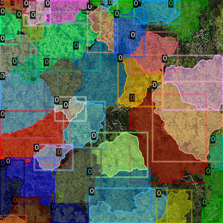
It is recommended to visually inspect the tiles before training to ensure that the tiling has worked as expected and
that crowns and images align. This can be done with the inbuilt detectron2 visualisation tools. For RGB tiles
(.png), the following code can be used to visualise the training data.
from detectron2.data import DatasetCatalog, MetadataCatalog
from detectron2.utils.visualizer import Visualizer
from detectree2.models.train import combine_dicts, register_train_data
import random
import cv2
from PIL import Image

name = "Danum"
train_location = "/content/drive/Shareddrives/detectree2/data/" + name + "/tiles_" + appends + "/train"
dataset_dicts = combine_dicts(train_location, 1) # The number gives the fold to visualise
trees_metadata = MetadataCatalog.get(name + "_train")

for d in dataset_dicts:
   img = cv2.imread(d["file_name"])
   visualizer = Visualizer(img[:, :, ::-1], metadata=trees_metadata, scale=0.3)
   out = visualizer.draw_dataset_dict(d)
   image = cv2.cvtColor(out.get_image()[:, :, ::-1], cv2.COLOR_BGR2RGB)
   display(Image.fromarray(image))
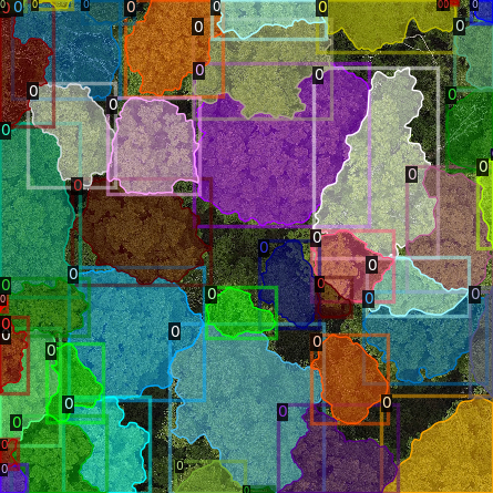
Alternatively, with some adaptation the detectron2 visualisation tools can also be used to visualise the
multispectral (.tif) tiles.
import rasterio
from detectron2.utils.visualizer import Visualizer
from detectree2.models.train import combine_dicts
from detectron2.data import DatasetCatalog, MetadataCatalog
from PIL import Image
import numpy as np
import cv2
import matplotlib.pyplot as plt
from IPython.display import display

val_fold = 1
name = "Paracou"
tiles = "/tilesMS_" + appends + "/train"
train_location = "/content/drive/MyDrive/WORK/detectree2/data/" + name + tiles
dataset_dicts = combine_dicts(train_location, val_fold)
trees_metadata = MetadataCatalog.get(name + "_train")

# Function to normalize and convert multi-band image to RGB if needed
def prepare_image_for_visualization(image):
   if image.shape[2] == 3:
      # If the image has 3 bands, assume it's RGB
      image = np.stack([
            cv2.normalize(image[:, :, i], None, 0, 255, cv2.NORM_MINMAX)
            for i in range(3)
      ], axis=-1).astype(np.uint8)
   else:
      # If the image has more than 3 bands, choose the first 3 for visualization
      image = image[:, :, :3]  # Or select specific bands
      image = np.stack([
            cv2.normalize(image[:, :, i], None, 0, 255, cv2.NORM_MINMAX)
            for i in range(3)
      ], axis=-1).astype(np.uint8)

   return image

# Visualize each image in the dataset
for d in dataset_dicts:
   with rasterio.open(d["file_name"]) as src:
      img = src.read()  # Read all bands
      img = np.transpose(img, (1, 2, 0))  # Convert to HWC format
      img = prepare_image_for_visualization(img)  # Normalize and prepare for visualization

   visualizer = Visualizer(img[:, :, ::-1]*10, metadata=trees_metadata, scale=0.5)
   out = visualizer.draw_dataset_dict(d)
   image = out.get_image()[:, :, ::-1]
   display(Image.fromarray(image))
2.3. Training (RGB)
Before training can commence, it is necessary to register the training data. It is possible to set a validation fold for model evaluation (which can be helpful for tuning models). The validation fold can be changed over different training steps to expose the model to the full range of available training data. Register as many different folders as necessary
train_location = "/content/drive/Shareddrives/detectree2/data/Danum/tiles_" + appends + "/train/"
register_train_data(train_location, 'Danum', val_fold=5)

train_location = "/content/drive/Shareddrives/detectree2/data/Paracou/tiles_" + appends + "/train/"
register_train_data(train_location, "Paracou", val_fold=5)
The data will be registered as <name>_train and <name>_val (or Paracou_train and Paracou_val in the
above example). It will be necessary to supply these registration names below…
We must supply a base_model from Detectron2’s model_zoo. This loads a backbone that has been pre-trained which
saves us the pain of training a model from scratch. We are effectively transferring this model and (re)training it on
our problem for the sake of time and efficiency. The trains and tests variables containing the registered
datasets should be tuples containing strings. If just a single site is being used a comma should still be supplied (e.g.
trains = ("Paracou_train",)) otherwise the data loader will malfunction.
# Set the base (pre-trained) model from the detectron2 model_zoo
base_model = "COCO-InstanceSegmentation/mask_rcnn_R_101_FPN_3x.yaml"

trains = ("Paracou_train", "Danum_train", "SepilokEast_train", "SepilokWest_train") # Registered train data
tests = ("Paracou_val", "Danum_val", "SepilokEast_val", "SepilokWest_val") # Registered validation data

out_dir = "/content/drive/Shareddrives/detectree2/240809_train_outputs"

cfg = setup_cfg(base_model, trains, tests, workers = 4, eval_period=100, max_iter=3000, out_dir=out_dir) # update_model arg can be used to load in trained  model
Note
tile_data also supports tile_placement (“grid” or “adaptive”) and options such as
overlapping_tiles and ignore_bands_indices. The defaults match prior behavior, so existing
examples continue to work, but you can use these parameters to better control tiling when needed.
Alternatively, it is possible to train from one of detectree2’s pre-trained models. This is normally recommended and
especially useful if you only have limited training data available. To retrieve the model from the repo’s
model_garden run e.g.:
!wget https://zenodo.org/records/10522461/files/230103_randresize_full.pth
Then set up the configurations as before but with the trained model also supplied:
# Set the base (pre-trained) model from the detectron2 model_zoo
base_model = "COCO-InstanceSegmentation/mask_rcnn_R_101_FPN_3x.yaml"

# Set the updated model weights from the detectree2 pre-trained model
trained_model = "./230103_randresize_full.pth"

trains = ("Paracou_train", "Danum_train", "SepilokEast_train", "SepilokWest_train") # Registered train data
tests = ("Paracou_val", "Danum_val", "SepilokEast_val", "SepilokWest_val") # Registered validation data

out_dir = "/content/drive/Shareddrives/detectree2/240809_train_outputs"

cfg = setup_cfg(base_model, trains, tests, trained_model, workers = 4, eval_period=100, max_iter=3000, out_dir=out_dir) # update_model arg used to load in trained model
Note
You may want to experiment with how you set up the cfg. The variables can make a big difference to how quickly
model training will converge given the particularities of the data supplied and computational resources available.
Once we are all set up, we can get commence model training. Training will continue until a specified number of
iterations (max_iter) or until model performance is no longer improving (“early stopping” via patience). The
patience parameter sets the number of training epochs to wait for an improvement in validation accuracy before
stopping training. This is useful for preventing overfitting and saving time. Each time an improved model is found it is
saved to the output directory.
Training outputs, including model weights and training metrics, will be stored in out_dir.
trainer = MyTrainer(cfg, patience = 5)
trainer.resume_or_load(resume=False)
trainer.train()
Note
Early stopping is implemented and will be triggered by a sustained failure to improve on the performance of predictions on the validation fold. This is measured as the AP50 score of the validation predictions.
2.4. Training (multispectral)
The process for training a multispectral model is similar to that for RGB data but there are some key steps that are
different. Data will be read from .tif files of 4 or more bands instead of the 3-band .png files.
Data should be registered as before:
from detectree2.models.train import register_train_data, remove_registered_data
val_fold = 5
appends = "40_30_0.6"
site_path = "/content/drive/SharedDrive/detectree2/data/Paracou"
train_location = site_path + "/tilesMS_" + appends + "/train/"
register_train_data(train_location, "ParacouMS", val_fold)
The number of bands can be checked with rasterio:
import rasterio
import os
import glob

# Read in geotif and assess mean and sd for each band
#site_path = "/content/drive/MyDrive/WORK/detectree2/data/Paracou"
folder_path = site_path + "/tilesMS_" + appends + "/"

# Select path of first .tif file
img_paths = glob.glob(folder_path + "*.tif")
img_path = img_paths[0]

# Open the raster file
with rasterio.open(img_path) as dataset:
   # Get the number of bands
   num_bands = dataset.count

# Print the number of bands
print(f'The raster has {num_bands} bands.')
Due to the additional bands, the weights of the first convolutional layer (conv1) are modified to accommodate a
variable number of input channels. This is automatically done in the case of imgmode being set to "ms"
and the update_model’s input channels not matching the current model’s.
The first three input weights are repeated across the new bands. The extension of the cfg.MODEL.PIXEL_MEAN
and cfg.MODEL.PIXEL_STD lists to include the additional bands happens within the setup_cfg function when
num_bands is set to a value greater than 3. imgmode should be set to "ms" to ensure the correct
training routines are called.
from datetime import date
import torch.nn as nn
import torch.nn.init as init
from detectron2.modeling.roi_heads.fast_rcnn import FastRCNNOutputLayers
import numpy as np
from detectree2.models.train import MyTrainer, setup_cfg

# Good idea to keep track of the date if producing multiple models
today = date.today()
today = today.strftime("%y%m%d")

names = ["ParacouMS",]

trains = (names[0] + "_train",)
tests = (names[0] + "_val",)
out_dir = "/content/drive/SharedDrive/detectree2/models/" + today + "_ParacouMS"

base_model = "COCO-InstanceSegmentation/mask_rcnn_R_101_FPN_3x.yaml"  # Path to the model config

# Set up the configuration
cfg = setup_cfg(base_model, trains, tests, workers = 2, eval_period=50,
               base_lr = 0.0003, backbone_freeze=0, gamma = 0.9,
               max_iter=500000, out_dir=out_dir, resize = "rand_fixed", imgmode="ms",
               num_bands= num_bands) # update_model arg can be used to load in trained  model
With additional bands, more data is being passed through the network per image so it may be neessary to reduce the
number of images per batch. Only do this is you a getting warnings/errors about memory usage (e.g.
CUDA out of memory) as it will slow down training.
cfg.SOLVER.IMS_PER_BATCH = 1
Training can now commence as before:
trainer = MyTrainer(cfg, patience = 5)
trainer.resume_or_load(resume=False)
trainer.train()
2.5. Data augmentation
Data augmentation is a technique used to artificially increase the size of the training dataset by applying random
transformations to the input data. This can help improve the generalization of the model and reduce overfitting. The
detectron2 library provides a range of data augmentation options that can be used during training. These include
random flipping, scaling, rotation, and color jittering.
Additionally, resizing of the input data can be applied as an augmentation technique. This can be useful when training a model that should be flexible with respect to tile size and resolution.
By default, random rotations and flips will be performed on input images.
augmentations = [
   T.RandomRotation(angle=[0, 360], expand=False),
   T.RandomFlip(prob=0.5, horizontal=True, vertical=False),
]
If the input data is RGB, additional augmentations will be applied to adjust the brightness, contrast, saturation, and lighting of the images. These augmentations are only available for RGB images and will not be applied to multispectral.
There are three resizing modes for the input data (1) fixed, (2) random, and (3) rand_fixed. This are set
in the configuration file (cfg) with the setup_cfg function.
The fixed mode will resize the input data to a images width/height of 1000 pixels. This is efficient but may not
lead to models that transfer well across scales (e.g. if the model is to be used on a range of different resolutions).
if cfg.RESIZE == "fixed":
   augmentations.append(T.ResizeShortestEdge([1000, 1000], 1333))
The random mode will randomly resize (and resample to change the resolutions) the input data to between 0.6 and 1.4
times the original height/width. This can help the model learn to detect objects at different scales and from images of
different resolutions (and sensors).
elif cfg.RESIZE == "random":
   size = None
   for i, datas in enumerate(DatasetCatalog.get(cfg.DATASETS.TRAIN[0])):
         location = datas['file_name']
         try:
            # Try to read with cv2 (for RGB images)
            img = cv2.imread(location)
            if img is not None:
               size = img.shape[0]
            else:
               # Fall back to rasterio for multi-band images
               with rasterio.open(location) as src:
                     size = src.height  # Assuming square images
         except Exception as e:
            # Handle any errors that occur during loading
            print(f"Error loading image {location}: {e}")
            continue
         break

   if size:
         print("ADD RANDOM RESIZE WITH SIZE = ", size)
         augmentations.append(T.ResizeScale(0.6, 1.4, size, size))
The rand_fixed mode constrains the random resizing to a fixed pixel width/height range (regardless of the resolution
of the input data). This can help to speed up training if the input tiles are high resolution and pushing up against
available memory limits. It retains the benefits of random resizing but constrains the range of possible sizes.
elif cfg.RESIZE == "rand_fixed":
      augmentations.append(T.ResizeScale(0.6, 1.4, 1000, 1000))
Which resizing option is selected depends on the problem at hand. A more precise delineation can be generated if high resolution images are retained but this comes at the cost of increased memory usage and slower training times. If the model is to be used on a range of different resolutions, random resizing can help the model learn to detect objects at different scales.
2.6. Post-training (check convergence)
It is important to check that the model has converged and is not overfitting. This can be done by plotting the training
and validation loss over time. The detectron2 training routine will output a metrics.json file that can be used
to plot the training and validation loss. The following code can be used to plot the loss:
import json
import matplotlib.pyplot as plt
from detectree2.models.train import load_json_arr

#out_dir = "/content/drive/Shareddrives/detectree2/models/230103_resize_full"
experiment_folder = out_dir

experiment_metrics = load_json_arr(experiment_folder + '/metrics.json')

plt.plot(
   [x['iteration'] for x in experiment_metrics if 'validation_loss' in x],
   [x['validation_loss'] for x in experiment_metrics if 'validation_loss' in x], label='Total Validation Loss', color='red')
plt.plot(
   [x['iteration'] for x in experiment_metrics if 'total_loss' in x],
   [x['total_loss'] for x in experiment_metrics if 'total_loss' in x], label='Total Training Loss')

plt.legend(loc='upper right')
plt.title('Comparison of the training and validation loss of detectree2')
plt.ylabel('Total Loss')
plt.xlabel('Number of Iterations')
plt.show()
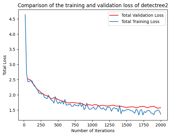
Training loss and validation loss decreased over time. As training continued, the validation loss flattened whereas the
training loss continued to decrease. The patience mechanism prevented training from continuing after 3000 iterations
preventing overfitting. If validation loss is substantially higher than training loss, the model may be overfitted.
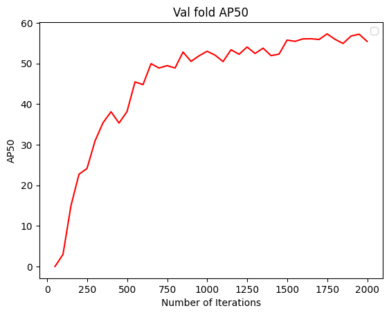
To understand how the segmentation performance improves through training, it is also possible to plot the AP50 score (see below for definition) over the iterations. This can be done with the following code:
plt.plot(
   [x['iteration'] for x in experiment_metrics if 'validation_loss' in x],
   [x['validation_loss'] for x in experiment_metrics if 'validation_loss' in x], label='Total Validation Loss', color='red')
plt.plot(
   [x['iteration'] for x in experiment_metrics if 'total_loss' in x],
   [x['total_loss'] for x in experiment_metrics if 'total_loss' in x], label='Total Training Loss')

plt.legend(loc='upper right')
plt.title('Comparison of the training and validation loss of detectree2')
plt.ylabel('Total Loss')
plt.xlabel('Number of Iterations')
plt.show()
2.7. Performance metrics
In instance segmentation, AP50 refers to the Average Precision at an Intersection over Union (IoU) threshold of 50%.
Precision: Precision is the ratio of correctly predicted positive objects (true positives) to all predicted bjects (both true positives and false positives).
Formula: \(\text{Precision} = \frac{\text{True Positives}}{\text{True Positives} + \text{False Positives}}\)
Recall: Recall is the ratio of correctly predicted positive objects (true positives) to all actual positive
objects in the ground truth (true positives and false negatives).
Formula: \(\text{Recall} = \frac{\text{True Positives}}{\text{True Positives} + \text{False Negatives}}\)
Average Precision (AP): AP is a common metric used to evaluate the performance of object detection and instance
segmentation models. It represents the precision of the model across various recall levels. In simpler terms, it is a combination of the model’s ability to correctly detect objects and how complete those detections are.
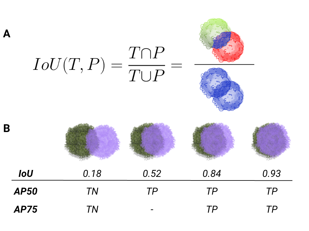
IoU (Intersection over Union): IoU measures the overlap between the predicted segmentation mask (or bounding box
in object detection) and the ground truth mask. It is calculated as the area of overlap divided by the area of union between the predicted and true masks.
AP50: Specifically, AP50 computes the average precision for all object classes at a threshold of 50% IoU.
This means that a predicted object is considered correct (a true positive) if the IoU between the predicted and ground truth masks is greater than or equal to 0.5 (50%). It is a relatively lenient threshold, focusing on whether the detected objects overlap reasonably with the ground truth, even if the boundaries aren’t perfectly aligned.
In summary, AP50 evaluates how well a model detects objects with a 50% overlap between the predicted and ground truth masks in instance segmentation tasks.
2.8. Evaluating model performance
Coming soon! See Colab notebook for example routine (detectree2/notebooks/colab/evaluationJB.ipynb).
2.9. Generating landscape predictions
Here we call the necessary functions.
from detectree2.preprocessing.tiling import tile_data
from detectree2.models.outputs import project_to_geojson, stitch_crowns, clean_crowns
from detectree2.models.predict import predict_on_data
from detectree2.models.train import setup_cfg
from detectron2.engine import DefaultPredictor
import rasterio
Start by tiling up the entire orthomosaic so that a crown map can be made for the entire landscape. Tiles should be approximately the same size as those trained on (typically ~ 100 m). A buffer (here 30 m) should be included so that we can discard partial the crowns predicted at the edge of tiles.
# Path to site folder and orthomosaic
site_path = "/content/drive/Shareddrives/detectree2/data/BCI_50ha"
img_path = site_path + "/rgb/2015.06.10_07cm_ORTHO.tif"
tiles_path = site_path + "/tilespred/"

# Location of trained model
model_path = "/content/drive/Shareddrives/detectree2/models/220629_ParacouSepilokDanum_JB.pth"

# Specify tiling
buffer = 30
tile_width = 40
tile_height = 40
tile_data(img_path, tiles_path, buffer, tile_width, tile_height, dtype_bool = True)
Warning
If tiles are outputting as blank images set dtype_bool = True in the tile_data function. This is a bug
and we are working on fixing it. Avoid supplying crown polygons otherwise the function will run as if it is tiling
for training.
To download a pre-trained model from the model_garden you can run wget on the package repo
!wget https://zenodo.org/records/10522461/files/230103_randresize_full.pth
Point to a trained model, set up the configuration state and make predictions on the tiles.
trained_model = "./230103_randresize_full.pth"
cfg = setup_cfg(update_model=trained_model)
predict_on_data(tiles_path, predictor=DefaultPredictor(cfg))
Once the predictions have been made on the tiles, it is necessary to project them back into geographic space.
project_to_geojson(tiles_path, tiles_path + "predictions/", tiles_path + "predictions_geo/")
To create a useful outputs it is necessary to stitch the crowns together while handling overlaps in the buffer. Invalid geometries may arise when converting from a mask to a polygon - it is usually best to simply remove these. Cleaning the crowns will remove instances where there is large overlaps between predicted crowns (removing the predictions with lower confidence).
crowns = stitch_crowns(tiles_path + "predictions_geo/", 1)
clean = clean_crowns(crowns, 0.6, confidence=0) # set a confidence>0 to filter out less confident crowns
By default the clean_crowns function will remove crowns with a confidence of less than 20%. The above ‘clean’ crowns
includes crowns of all confidence scores (0%-100%) as confidence=0. It is likely that crowns with very low
confidence will be poor quality so it is usually preferable to filter these out. A suitable threshold can be determined
by eye in QGIS or implemented as single line in Python. Confidence_score is a column in the crowns GeoDataFrame
and is considered a tunable parameter.
clean = clean[clean["Confidence_score"] > 0.5] # step included for illustration - can be done in clean_crowns func
The outputted crown polygons will have many vertices because they are generated from a mask which is pixelwise. If you
will need to edit the crowns in QGIS it is best to simplify them to a reasonable number of vertices. This can be done
with simplify method. The tolerance will determine the coarseness of the simplification it has the same units as
the coordinate reference system of the GeoSeries (meters when working with UTM).
clean = clean.set_geometry(clean.simplify(0.3))
Once we’re happy with the crown map, save the crowns to file.
clean.to_file(site_path + "/crowns_out.gpkg")
View the file in QGIS or ArcGIS to see whether you are satisfied with the results. The first output might not be perfect and so tweaking of the above parameters may be necessary to get a satisfactory output.